Investigate the APO and HOLO mu-Opioid receptor
Introduction
This guide will provide a brief overview of a G protein-coupled receptor (GPCR) system. GPCRs are membrane-embedded proteins that mediate signalling across lipid bilayers by detecting molecules outside the cell and activating the corresponding intra-cellular responses. They are characterized by seven trans-membrane \(\alpha\) helices that pass through the cell membrane with the N-terminal in the extracellular region and the C-terminal in the intracellular one. There are several classes of GPCRs, but here we focus on a class A GPCR, the mu-opioid receptor (Wang et al. 2023; Vigneron et al. 2025) (or muOR). The muOR receptor occupies a pivotal role in pain modulation and reward circuitry, and is the principal target of clinically used opioid analgesics such as morphine and fentanyl. muOR is involved in mediating the therapeutic effects and major liabilities of these drugs, which include respiratory depression, tolerance, dependence, and addiction. Thus, muOR is both a critical drug target and a receptor of exceptional public health relevance.
The activation mechanism of Class A GPCRs typically involves the binding of a ligand to an extracellular binding site, which induces a conformational shift towards active states that facilitates recruitment of effectors, e.g. G-proteins and arrestins, at the intracellular effector binding site. Effectors such as the G-proteins propagate the signal onward, while arrestins typically terminate G-protein signalling by preventing further G-protein coupling and promoting receptor internalization. The activation of GPCRs entails a complex network of coordinated conformational rearrangements within the receptor itself. Both structural transitions and ligand binding can’t usually be obtained with normal unbiased MD simulations (but can be induced with enhanced sampling (Aureli et al. 2026)). Nevertheless, the difference between APO and HOLO states can still be easily observed if these crystals are available.
Despite being trans-membrane proteins, i.e., systems in which the lipid scaffolding is fundamental to their functioning, GPCR experimental structures are generally published without the embedding lipid bilayer, although sometimes lipid molecules bound to specific GPCR binding sites are resolved, as shown here in Figure 1 in the \(\beta\)-adrenergic receptor, another Class A GPCR.
Nowadays, there are well-established procedures to embed proteins in lipid bilayer and thus properly simulate the (closest) physiological state of these system, arguably the most known being CHARMM-GUI webserver. Nevertheless, to better focus on how to set up the simulation box to get the simulations going and analyze data, the starting structure provided in this tutorial is already embedded in a mixed lipid bilayer of cholesterol and phosphatidylcholine (POPC), a common mixture for cell membrane simulations.
A look into the starting files
First of all, start by downloading the exercise directories from the github repository.
We provide three different systems. These are always the same protein (muOR) but in different states, i.e., ligand-less (APO) or ligand-bound (HOLO) with two different molecules, endomorphine (ENDO) and buprenorphine (BPN). You should download and run simulations of at least two of them, one being the APO and one a HOLO so that you can compare the structures at the end of the molecular dynamics simulation. You can unzip the downloaded directories with the command
tar -xvf name_of_compressed_file.tar.gzThe individual directories of the different structures are organized as in the following
muOR_APO/HOLO_X_exercise
│   ionize.mdp
│   reference_topology_MUOR_X.gro
│   reference_topology_MUOR_X.top
│   sbatch_me.sh
│   water_removal.py
│
└─── forcefield
│   │   [various forcefields files]
│
└─── step1_em
│   │   em.mdp
│
└─── step2_nvt
│   │   [various nvt.mdp files]
│
└─── step3_npt
│   │   [various npt.mdp files]
│
└─── step4_prod
    │   prod.mdp
Going by order, you can see
The
ionize.mdp,reference_topology_MUOR_X.gro,reference_topology_MUOR_X.top, andwater_removal.pyfiles. These are the building blocks to set up your starting configuration. These will be covered in depth later in this tutorial;A
sbatch_me.shfile. This is a text file that contains the set of instructions that will run your starting configuration through energy minimization, NVT, NPT, and eventually the production phase;A
forcefielddirectory. Inside this, you can find several text files that define ‘numerically’ the key components of your system. You might recognize some of them, likeMUOR.itp,cholesterol.itp, andPOPC.itp. You can peek inside them and take a look at how a molecule is described numerically in MD simulations. The format of these files - that is, how these numbers are organized and reported - depends on the software you are using. Since in this course you use GROMACS, these files are written in GROMACS format. However, while these numbers and these files might be different for other softwares, the core idea of numerically representing with specific functions the intra- and inter-molecular interactions is paramount in molecular dynamics;The
step1_em,step2_nvt, andstep3_nptdirectories. Inside each of these you can find one or moremdp(molecular dynamics parameters) files that will be used to compile and run the energy minimization, the NVT, and the NPT equilibrations. These will be run sequentially by the scriptsbatch_me.sh, taking your starting configuration through a set of equilibration phases to relax the starting configuration gradually and avoid the system exploding;The
step4_proddirectory. Here there is theprod.mdpfile, which is the final mdp file for the production run of the system. This is usually the longest part of the simulation, which can take 2 to 4 days on Baobab depending on the system. The final output files of the simulation will be inside this directory, and the analysis for the exam will mainly revolve around theprod.xtctrajectory file.
The idea of this tutorial is to give you the main ingredients to build your own solvated simulation box without going through the hassle of finding a good target to simulate, fix the experimental structure files, find a consistent force field to describe the system, and embedding the protein in the membrane. Considering this, inside the main directory you can find a copy of four files which will be the basic blocks to build the system, namely
ionize.mdp, the mdp file to add the ions in the system;reference_topology_MUOR_X.gro, the starting structure that contains the trans-membrane domain of the muOR already embedded in the membrane with the ligand (if present);reference_topology_MUOR_X.top, the starting topology of the system;water_removal.py, a python script that removes the water molecules that GROMACS wrongly positions within the lipid bilayer during the solvation phase.
From these, and if needed by using as reference the Lysozyme in water tutorial for solvation and ion addition, you should be able to obtain three files, that is the starting configuration of the solvated membrane, which you will name start.gro, the updated topology of the system, which you will name topol.top, and the index file of the system, which you will name index.ndx, which is a useful tool for better controlling complex multi-phase systems like a protein embedded in a lipid bilayer. These files will be then picked up by the sbatch_me.sh script and used as starting point to run the equilibration and the production runs of the system.
The rest of this tutorial will show the set-up of the simulation box by using as example the HOLO+ENDO system. Nevertheless, the logic of the procedure is identical and can be applied directly to all the other systems as well.
Preparing the HPC environment
Login into Baobab and send the directory with the exercises to your home in Baobab (with scp), or directly download it there (with wget). Then, request a node with and interactive job for a couple of hours with salloc in the following way
salloc --ntasks=1 --cpus-per-task=4 --partition=private-gervasio-cpu --time=120:00Finally, source the GROMACS installation
module load GCC/11.3.0
module load OpenMPI/4.1.4
module load GROMACS/2023.1-CUDA-11.7.0
and verify that the sourcing was okay by typing
gmx --versionYou are now ready to assemble the starting configuration of the system.
Notice how here you are requesting 4 CPUs but no GPU, differently from the HPC tutorial (in fact, you are on --partition=private-gervasio-cpu). In this case, you are going to use the allocation on Baobab just to set up the box and not to run the simulation, so the GPU is not needed.
GROMACS has a lot (> 100) of tools that are accessible by typing gmx followed by a keyword. In this tutorial you will use solvate, grompp, genion, and make_ndx. If you have any doubts remember that you can look online for the explanation of the tool and which flags are needed (-f, -o, -s etc.). For example, this is the manual page of gmx solvate. All this information is also available on the spot if you type -h or --h (for help) after the tool’s name, e.g., gmx solvate --h.
Solvating
At the beginning, you can take a look at the starting topology (reference_topology_MUOR_ENDO.top) and the starting configuration to solvate (reference_topology_MUOR_ENDO.gro). The topology reads like this
#include "./forcefield/forcefield.itp"
#include "./forcefield/cholesterol.itp"
#include "./forcefield/MUOR.itp"
#include "./forcefield/ENDO.itp"
#include "./forcefield/POPC.itp"
#include "./forcefield/tip4pd.itp"
#include "./forcefield/ions.itp"

[ system ]
; Name
MUOR HOLO ENDO

[ molecules ]
; Compound        #mols
MUOR                1
ENDO                1
CHL                64
POPC              256
First of all, notice that sometimes there are lines starting with a semi-column ;. These are comments, that is, lines that are not read by GROMACS. Comments are used to annotate the files and write down details that are helping you - the users - remember what you are doing, what is the meaning of some variables, etc. They are ignored by the software and should be informative for the person writing or for the person supposed to read the code. Feel free to write your own comments, if it helps you, just remember to put a ; at the beginning of each line that you do not want to be read by GROMACS, otherwise you will receive a fatal error.
Following up, the #include statements tell GROMACS where to find the elements of the force field. As can be seen, they are collected inside the forcefield directory and must appear with a specific order. First, the set of parameters defining the force field (forcefield.itp). Then, the definition of the individual molecules (cholesterol.itp, GPCR.itp, etc.) that will populate your system. These do not have to appear in a specific order, however all the molecules that you intend to use must be defined here. Building the topology, that is, filling in this file, is roughly the equivalent of running gmx pdb2gmx on the pdb file of the protein, as you did in the Lysozyme tutorial. After the the #include statements, there is the [ system ] section, which is simply the name of the system. It is worth giving the system a meaningful name to help in recognizing the systems in the future.
Finally, there is the [ molecules ] section, which must contain all the molecules of the system in the order in which they appear in the box. Notice that, for the time being, the topology contains the muOR, the ligand (ENDO for endomorphine), 64 cholesterol molecules (CHL), and 256 phospholipids (POPC).
GROMACS (and other modelling software) doesn’t know if a ligand necessitates some ions and coordinating water molecules. Thus, they are part of the initial box before the solvation as they have been modelled already in the correct state. This is where the biological and chemical knowledge of the user is critical for building a physiologically correct system. Among the systems presented in this tutorial, there is no ligand that necessitates other molecules to be modelled properly in its binding site. Other important paramenters to consider if you prepare a system are the protonation state of both the ligand and the protein, the binding pose of the ligand, eventual missing structural sections of the protein that need to be modelled by hand, mutations that need to be back-mutated and so on.
The APO structure and the two ligands are shown in the panels of Figure 2.
Now, take a look at the starting configuration reference_topology_MUOR_ENDO.gro. The .gro file has a fixed format, and it is better to not modify it by hand if you are not completely sure about what you are doing. The top of the file looks like this
MUOR HOLO ENDO
43865
    1ACE    CH3    1   3.289   5.610   2.425
    1ACE   HH31    2   3.378   5.555   2.394
    1ACE   HH32    3   3.240   5.653   2.338
    1ACE   HH33    4   3.228   5.533   2.474
    1ACE      C    5   3.301   5.713   2.542
    1ACE      O    6   3.375   5.697   2.643
    2MET      N    7   3.236   5.825   2.525
[...]
The first line contains the title of the box (MUOR HOLO ENDO), the second line contains the number of the atoms in the box (43865), and the following ones report in order all the atoms of the system. These are organized usually as nine columns. The first (here 1ACE) is the specific number and name of the residue, which in this case is the capped N-terminal of the protein. The second column contains the specific name of the atom, and usually the first letter indicates the element (here you have a carbon followed by three hydrogen and a carbon and so on). The third is simply the number of the entry. It always starts with 1 and goes up to the number of elements in the box. Then, columns four to six contain the x, y, and z coordinates of that atom, while the columns seven to nine contain its velocity, reported by axial component. All atoms must always have a position, but might have zero -or not reported- velocity, like here. One of the main roles of the equilibrations phase is this - to relax the starting positions and assign reasonable starting velocities to all the atoms.
At the other end of the file, the last lines look like this
[...]
615POPC H17S43861 1.937 0.190 3.981
615POPC C11843862 2.133 0.174 4.056
615POPC H18R43863 2.135 0.276 4.094
615POPC H18S43864 2.238 0.153 4.036
615POPC H18T43865 2.116 0.120 4.149
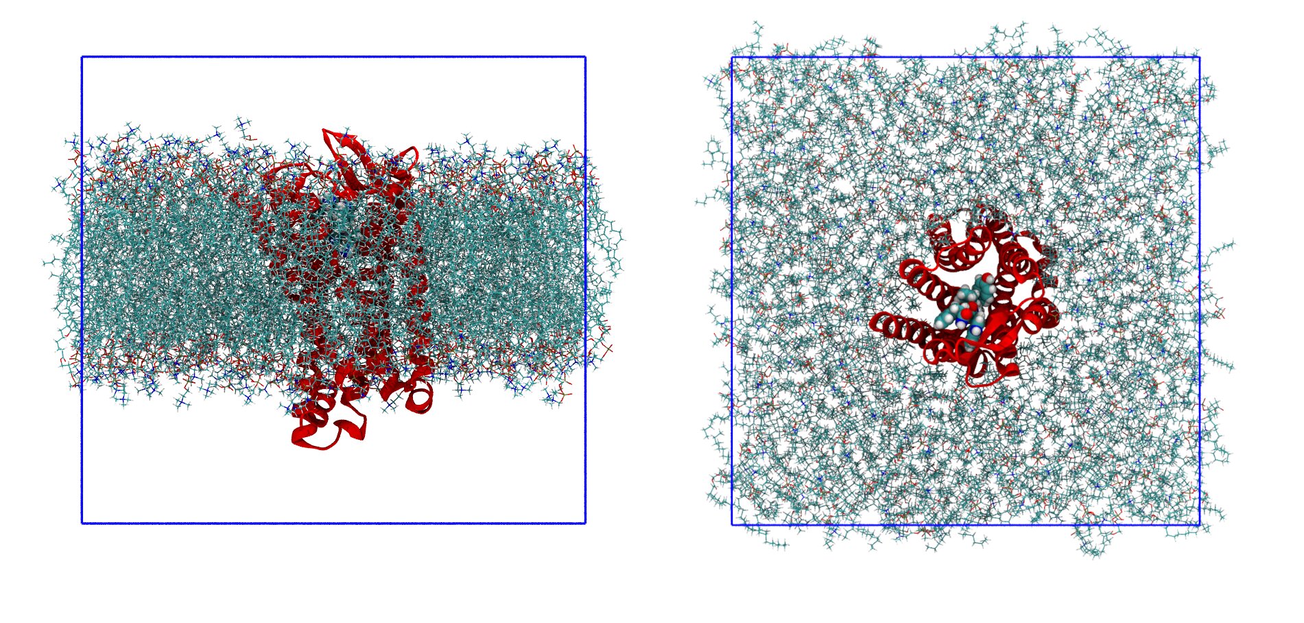
10.15889 10.15889 9.41398The meaning of the columns is the same as before. The last molecules to appear are the phopsholipids (and in fact, in the topology, they are reported last). The last line of a .gro file has, like the first two, a special meaning, as it reports the side length of the box along x, y, and z. For example, this box is roughly a cube, with x and y lengths of 10.15889 nm and z length of 9.41398 nm. Sometimes, for special types of boxes (like those used for the protein-ligand simulations), there might be more than three values reported. The starting configuration, which you can visualize with VMD, is reported in Figure 3.
The first step is then to solvate the system. In the Lysozyme tutorial, before solvation, the gmx editconf command is used to prepare the box and to make it large enough to fit the protein. Here, you do not use it as the box is already prepared because it depends on the width of the lipid bilayer.
Before running gmx solvate, you have to know which water model you want to use. For this force field, as also reported in the reference_topology_MUOR_ENDO.top file, the model is TIP4PD (you are importing the parameters with this line #include "./forcefield/tip4pd.itp"), a four-point water model. This means that each water molecule in your simulation will be actually represented with four sites: one oxygen atom, two hydrogen atoms, and a dummy site near the oxygen atom that has negative charge. This dummy atom is a numerical trick to better represent the distribution of charge of the lone pair in water’s oxygen. To access four-points water models, the flag name for gmx solvate is -cs tip4p.gro.
Thus, you can solvate the system with the following
gmx solvate -cp reference_topology_MUOR_ENDO.gro -cs tip4p.gro -o MUOR_ENDO_solvated.growhere you are asking to add water to the structure with -cp reference_topology_MUOR_ENDO.gro, use as reference a four-points water model with -cs tip4p.gro, add call the resulting output structure -o MUOR_ENDO_solvated.gro. Some of you may notice that in the Lysozyme tutorial you also have to pass the topology of the system with the -p flag. This is not mandatory, but if you pass it then the updated topology will have the same name as the input one, which makes things harder to trace back if something goes wrong. However, if you do not pass the topology, you will have to update it by hand to include the presence of the water molecules.
The (last lines of the) output of the solvate command will look something like this
[...]
Volume                 :     971.551 (nm^3)
Density                :     1007.58 (g/l)
Number of solvent molecules:  18525
GROMACS tries to fill the box with water to reach the density of ca. 1g/L. The most important part here is the number of water molecules inserted, in this case 18525 (this number can oscillate slightly, as molecules are randomly inserted). In principle, you could add this number at the end of the topology and you would be done with the solvation, as in the Lysozyme tutorial. However, you might think that the system has actually more than one phase (lipids and protein) and that GROMACS tried to insert water molecules in each and every empty volume it could find. How did it behave near the protein and the lipids? You can check with VMD.
Removing additional water
The result after solvation is shown in Figure 4. Water has been inserted in all places where there was some spare free volume, also between the lipid leaflets, which is not realistic as this is an hydrophobic region. Generally, this is not a major problem, and within the first nanoseconds of run the water molecules get expelled naturally because of the chemical nature of the lipid tail region. Nevertheless, for delicate systems like this that involve proteins highly susceptible to non-physiological starting configurations, it is better to get rid of them and clean the system before adding the ions.
You can remove these wrongly placed water molecules with the water_removal.py Python script, which you can run with the following command
python3 water_removal.py MUOR_ENDO_solvated.gro MUOR_ENDO_solvated_clean.groThe script takes as input MUOR_ENDO_solvated.gro, check where there are overlapping water molecules with the lipids and the protein, removes them, and returns the cleaned system under the name MUOR_ENDO_solvated_clean.gro. The output looks something like this
Initial number of water molecules: 18525
Number of water molecules to be deleted: 1457
Final number of water molecules: 17068
The script removed ca. 1500 water molecules. You can see now, in Figure 4, that the system has been cleaned and looks much more biologically sound.

gmx solvate. On the right, the same system after removing ca. 1500 water molecules with the water_removal.py script. Notice how there are no more water molecules in the lipid bilayer. Protein, lipids and ligand are coloured as in Figure 3, while water molecules in red (oxygen) and white (hydrogen).
If you take a look at the MUOR_ENDO_solvated_clean.gro file, you will notice that the last lines will look like the following
[...]
19140SOL     OW17962  10.317   9.424   9.395
19140SOL    HW117963  10.373   9.416   9.317
19140SOL    HW217964  10.294   9.334   9.417
19140SOL     MW17965  10.322   9.411   9.388
  10.15889  10.15889   9.41398
where SOL is the name of the solvent molecules (water) and each SOL molecule has four atoms. The box size, as expected, didn’t change. When there are many atoms in the box, the space between the second and the third column might disappear. For example, OW17962 is an atom called OW and it’s the entry number 17962, but the space between is not present anymore. This also is not a problem sa long as the length of each field remains constant.
The first lines look like before exception made for the number of atoms, which now has been updated to contain also those of water (in fact the starting dry box had 43865 atoms to which you added 17068 four-point water molecules, that is 43865 + 17068 x 4 = 112137).
MUOR HOLO ENDO
112137
    1ACE    CH3    1   3.289   5.610   2.425
    1ACE   HH31    2   3.378   5.555   2.394
    1ACE   HH32    3   3.240   5.653   2.338
    1ACE   HH33    4   3.228   5.533   2.474
    1ACE      C    5   3.301   5.713   2.542
    1ACE      O    6   3.375   5.697   2.643
[...]
Now, you can update the topology. First, copy the reference topology and call it reference_topology_MUOR_ENDO_solvated.top
cp reference_topology_MUOR_ENDO.top reference_topology_MUOR_ENDO_solvated.topThen, add the amount of water molecules to reference_topology_MUOR_ENDO_solvated.top by correcting the [ molecules ] section
[...]
[ molecules ]
; Compound        #mols
MUOR                1
ENDO                1
CHL                64
POPC              256
SOL             17068
You have to add the name of the water in the box (SOL) and the number reported after cleaning up the system with the python script. At this point, the structure of the solvated system is contained in MUOR_ENDO_solvated_clean.gro, while its topology in reference_topology_MUOR_ENDO_solvated.top.
Adding ions
You are now ready to add the ions in the system. First, you need to generate a .tpr file, which is a binary file that GROMACS can read to understand the charges of the different molecules in the system and select automatically how many ions should be added. You can do this by using gmx grompp and pointing to the parameters file ionize.mdp with the flag -f, to the starting solvated structure MUOR_ENDO_solvated_clean.gro with the flag -c, to the solvated topology reference_topology_MUOR_ENDO_solvated.top with the flag -p, and finally name the output tpr file ionize.tpr with the flag -o
gmx grompp -f ionize.mdp -c MUOR_ENDO_solvated_clean.gro -p reference_topology_MUOR_ENDO_solvated.top -o ionize.tprYou might see (depending on GROMACS version) that for some systems the command fails with a fatal error containing the following information
NOTE 2 [file reference_topology_MUOR_ENDO_solvated.top, line 19]:
  System has non-zero total charge: 13.999743
  Total charge should normally be an integer. See
  http://www.gromacs.org/Documentation/Floating_Point_Arithmetic
  for discussion on how close it should be to an integer.

WARNING 1 [file reference_topology_MUOR_ENDO_solvated.top, line 19]:
  You are using Ewald electrostatics in a system with net charge. This can
  lead to severe artifacts, such as ions moving into regions with low
  dielectric, due to the uniform background charge. We suggest to
  neutralize your system with counter ions, possibly in combination with a
  physiological salt concentration.
Basically, a tpr file is used to run simulations. As such, when GROMACS tries to prepare one through gmx grompp, it check if the physics of the system is reasonable or not. In this case, it found that your system has a positive net charge, and is telling you that this is very bad as the systems should always have zero total net charge. You can bypass this check by adding the flag --maxwarn 1 to the command line, that is, ignore one (and only one) warning
gmx grompp -f ionize.mdp -c MUOR_ENDO_solvated_clean.gro -p reference_topology_MUOR_ENDO_solvated.top -o ionize.tpr -maxwarn 1You will see that now GROMACS still complains, but gets the job done. It is very important, however, to understand that the ionization step is nearly the only case in which it is okay to use the -maxwarn flag, as you know that the physics of the system is wrong and you actually need the tpr to fix it with gmx genion.
You may be temped to use -maxwarn to get through errors, but generally you should never use this flag without understanding the problem. If there is a major warning then you have to check what is happening. With -maxwarn you can compile the binary but the simulation will probably fail instantly the moment you try to run it, or, worse, it will run but you are likely to produce garbage results due to overlooking fundamental physics mistakes in the box preparation.
Now, you should have a ionize.tpr file in your directory, following the gmx grompp command. You are ready to insert the ions with the following command
gmx genion -s ionize.tpr -neutral -pname NA -nname CL -o start.groHere, you are asking GROMACS to make the system neutral (-neutral), call the positive ions NA, the negative ions CL, and call the resulting output start.gro. Trivially, within this force field the atoms NA and CL refer to sodium (Na, +1) and chlorine (Cl, -1) ions. Again, differently from the Lysozyme tutorial, you are not giving as input the topology and you will update it after the addition of ions.
With genion, GROMACS tries to substitute some molecules in the system with the necessary number of ions. You will be prompted by GROMACS to choose which part of the system you are okay to substitute in favour of water molecules
Will try to add 0 NA ions and 14 CL ions.
Select a continuous group of solvent molecules
Group     0 (         System) has 112137 elements
Group     1 (        Protein) has  4825 elements
Group     2 (      Protein-H) has  2367 elements
Group     3 (        C-alpha) has   292 elements
Group     4 (       Backbone) has   879 elements
Group     5 (      MainChain) has  1172 elements
Group     6 (   MainChain+Cb) has  1455 elements
Group     7 (    MainChain+H) has  1458 elements
Group     8 (      SideChain) has  3367 elements
Group     9 (    SideChain-H) has  1195 elements
Group    10 (    Prot-Masses) has  4825 elements
Group    11 (    non-Protein) has 107312 elements
Group    12 (          Other) has 39040 elements
Group    13 (            CHL) has  4736 elements
Group    14 (           POPC) has 34304 elements
Group    15 (          Water) has 68272 elements
Group    16 (            SOL) has 68272 elements
Group    17 (      non-Water) has 43865 elements
Select a group:
From the first line you can see that GROMACS understood that the system has a total of ca. +14 charge and will then need fourteen negative ions to have a total of ca. zero net charge. Since you do not want to substitute any part of the protein or lipids, choose the SOL group, and GROMACS will randomly choose seven water molecules, remove them and place there a chlorine ion.
Selected 16: 'SOL'
Number of (4-atomic) solvent molecules: 17068
Using random seed 1834818167.
Replacing solvent molecule 14306 (atom 101089) with CL
Replacing solvent molecule 15927 (atom 107573) with CL
Replacing solvent molecule 7440 (atom 73625) with CL
Replacing solvent molecule 6745 (atom 70845) with CL
Replacing solvent molecule 8092 (atom 76233) with CL
Replacing solvent molecule 12068 (atom 92137) with CL
Replacing solvent molecule 3940 (atom 59625) with CL
Replacing solvent molecule 564 (atom 46121) with CL
Replacing solvent molecule 10093 (atom 84237) with CL
Replacing solvent molecule 12948 (atom 95657) with CL
Replacing solvent molecule 2208 (atom 52697) with CL
Replacing solvent molecule 6294 (atom 69041) with CL
Replacing solvent molecule 10286 (atom 85009) with CL
Replacing solvent molecule 11481 (atom 89789) with CL
As for the solvation, you need now to update the topology as some water molecules have been removed and some chlorine ions have been added. Start by copying the solvated topology into a new topology called topol.top
cp reference_topology_MUOR_ENDO_solvated.top topol.topand change the [ molecules ] section by removing the seven water molecules from the total and adding the seven chlorine ions (CL)
[ molecules ]
; Compound        #mols
MUOR                1
ENDO                1
CHL                64
POPC              256
SOL             17054
CL 14Here you can notice that the charge is actually not an integer, as also pointed out by the Note during the generation of the tpr for ionisation. Non-integer charges should usually be avoided, as the addition of ions with integer charge cannot formally neutralize the system. In fact, the system’s charge of 13.999743 plus fourteen cloride ions of charge -1 will leave the system with a net charge of -0.000257. This is a by-product of a force field conversion (a porting of the des-Amber force field to GROMACS format), and it’s not optimal.
You have two options to overcome this problem. The first is to repartition the leftover charge, so redistribute it to some molecule in the box to reach net zero charge; the second is to proceed with leftover charge. Generally, the refactoring of the charge is very dangerous, and might not be simple for numerical reasons. Thus, a common approach -and the one we will use here- is to proceed anyway assuming that the leftover charge is so small that it impacts very little the dynamics of the system. Practically speaking, this means that all the times you will generate a tpr file with grompp you will have to -maxwarn 1 the warning due to the box’s small net charge.
Summarizing, you now have the starting solvated and neutralized configuration stored in start.gro and the corresponding topology in topol.top. You can take a look at the final system with VMD. It should look similar to that shown in Figure 5.
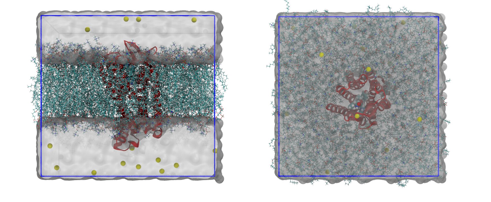
Life doesn’t happen in pure water. Generally, during the system preparation a certain amount of salt is added to reach a given physiological salt concentration. These ions are added on top of those needed to neutralize the system. If you want a more realistic set-up, you can ionize the system to 0.150 M with
gmx genion -s ionize.tpr -neutral -pname NA -nname CL -conc 0.150 -o start.grobut remember to update accordingly the topology with both NA and CL atoms.
Generate the index file
The last passage before running the simulation is, sometimes, to generate an index file. This type of file is used to name part of the system by grouping the corresponding atom numbers under a given name. In this case, you need an index file because the thermostat is expecting two different groups to couple for temperature regulation, one that contains the protein and the lipids, which you will call non-Solv, and one that contains the water and the ions, which you will call Water_and_ions. The reasons behind this are technical and go beyond the scope of this tutorial. However, the index file is a powerful tool to address only parts of the simulation box, and as such it is important to know how to generate one.
The command to generate an index file is make_ndx. As input you should give the final configuration and call the output simply index.ndx, as in the following
gmx make_ndx -f start.gro -o index.ndxGROMACS will answer by showing you what types of molecules it sees inside the box and which name it would give to them
  0 System              : 112095 atoms
  1 Protein             :  4825 atoms
  2 Protein-H           :  2367 atoms
  3 C-alpha             :   292 atoms
  4 Backbone            :   879 atoms
  5 MainChain           :  1172 atoms
  6 MainChain+Cb        :  1455 atoms
  7 MainChain+H         :  1458 atoms
  8 SideChain           :  3367 atoms
  9 SideChain-H         :  1195 atoms
 10 Prot-Masses         :  4825 atoms
 11 non-Protein         : 107270 atoms
 12 Other               : 39040 atoms
 13 CHL                 :  4736 atoms
 14 POPC                : 34304 atoms
 15 CL                  :    14 atoms
 16 Water               : 68216 atoms
 17 SOL                 : 68216 atoms
 18 non-Water           : 43879 atoms
 19 Ion                 :    14 atoms
 20 Water_and_ions      : 68230 atoms
A few of these groups are very important, e.g., group 1 is the protein, group 13 contains the cholesterol lipids while group 14 the POPC lipids, and so on. You can also see that GROMACS already puts together in a group water and ions (group 20, Water_and_ions). Thus, you will only need to generate another group that contains everything excluded water and ions, that is, the protein, the lipids, and the ligand. You can achieve this by typing
! 20and pressing enter. You can read the legend at the end of the list of groups to understand what you just did. You basically said to take everything that is not (!) inside group 20, so the protein, the ligand, and the membrane. If you press enter again, GROMACS will show the list of groups inside the index file, and you can see how now there is a new one at the end
[...]
 18 non-Water           : 43879 atoms
 19 Ion                 :    14 atoms
 20 Water_and_ions      : 68230 atoms
 21 !Water_and_ions     : 43865 atoms
which is the union of the protein with the lipids. You can rename it by typing
name 21 non-SolvPress enter again to confirm the command, and you will see now that the group changed name
[...]
 18 non-Water           : 43879 atoms
 19 Ion                 :    14 atoms
 20 Water_and_ions      : 68230 atoms
 21 non-Solv            : 43865 atoms
You can exit the index generation by typing q and pressing enter. In your main directory you should now have the starting configuration start.gro, the corresponding topology topol.top, and the index file that you just generated, index.ndx. This is all what you need to run the following simulations.
A look at the sbatch_me.sh file
The content of the exercise directory should now be similar to this
muOR_HOLO_ENDO_exercise
│   sbatch_me.sh
│   index.ndx
│   start.gro
│   topol.top
│
└─── forcefield
│
└─── step1_em
│   │   em.mdp
│
└─── step2_nvt
│   │   [various nvt.mdp files]
│
└─── step3_npt
│   │   [various npt.mdp files]
│
└─── step4_prod
    │   prod.mdp
plus some leftover files from the system generation. It is mandatory that sbatch_me.sh, index.ndx, start.gro, and topol.top are together in the same directory in which there are the energy minimization, NVT, NPT, and production directories, otherwise the script sbatch_me.sh won’t be able to run the simulations for you.
During both the Lysozyme tutorial and the preparation of the box for this exercise, you logged in a Baobab node by using the salloc command. In this way you can have access to a node and run an interactive job. This is nice because you can have real time answers from the node and you see clearly what is going on and what you are doing, which is pivotal for error-prone procedures like the generation of the starting box. However, when you close the connection, log out from Baobab, or simply turn off the computer, you lose the access to the computer and any running simulation will stop. Does this mean that you should be always connected? And that you should stay constantly in front of your computer, even for a few days at a time, while the simulations run, scared or losing the internet connection and see your runs fail?
Clearly this is not the case. As explained also in the Introduction to HPC, Baobab has a so-called queueing system, named slurm. With slurm, you can prepare a submission script that contains the main commands that you want to run alongside the resources you need. This is exactly what the sbatch_me.sh script is.
Take a look at the content of the sbatch_me.sh. The first lines look like this
#!/bin/bash

#SBATCH --account=gervasio_teach_19h330
#SBATCH --partition=private-gervasio-gpu
#SBATCH --time 144:00:00
#SBATCH --job-name muOR_ENDO
#SBATCH --error jobname-error.e%j
#SBATCH --output jobname-out.o%j
#SBATCH --ntasks 1
#SBATCH --cpus-per-task 16
#SBATCH --nodes 1
#SBATCH --gpus-per-node=nvidia_geforce_rtx_3080:1
#SBATCH --hint=nomultithread

[...]
You can recognise some of the flags that you were giving to the salloc command, such as --partition=private-gervasio-gpu and --cpus-per-task 16. Basically these lines are specifying which kind of hardware you need to run the simulations. If you are curious, you can look up their meaning in the slurm website.
Slurm reads this files and sends you in a queue while it waits to find some computer that is available and that has the requested hardware. When it finds it, it takes control for the amount of time specified in --time 144:00:00, that is, six days. This amount of time will be sufficient to both conclude the equilibration and the production runs.
Continuing along the sbatch_me.sh script, as in the interactive case, the first thing to do once the node is allocated is to source GROMACS, which is the first thing done by the script with the lines following the #SBATCH node requests, i.e., with the following
[...]
module load GCC/11.3.0
module load OpenMPI/4.1.4
module load CUDA/11.7.0
module load GROMACS/2023.1-CUDA-11.7.0
[...]
Then there are a few technical details about how GROMACS should use the available resources to run the simulations with gmx mdrun (e.g. -ntmpi, -ntomp, etc.). Lastly, there are a series of cd commands that enter the step1_em, step2_nvt, step3_npt, and step4_prod directories and systematically run gmx grompp to prepare the corresponding tpr files and then run them with gmx mdrun.
Notice that all the gmx grompp commands contain the -maxwarn 1 flag. This is due to the leftover charge from the ionization step which will raise a warning every time you compile a tpr with this topology.
You can send the submission script sbatch_me.sh and let slurm handle the simulations by using the sbatch command. This should be run from Baobab’s head-node, and not from the node that you received by running salloc. Thus, from the muOR_HOLO_X_exercise directory where the submission script sbatch_me.sh is located, you can submit the job slurm with the following command
sbatch sbatch_me.shIf the command runs successfully, slurm returns the number that is assigned to your job, something like this
Submitted batch job 7404228You can check the status of the job by running (and substituting username with yours)
squeue -u usernameThe output will look something like this
             JOBID PARTITION     NAME     USER ST       TIME  NODES NODELIST(REASON)
           7404228 private-g muOR_END username  R       0:47      1 gpu037
The R under the column ST (for status) stands for running. Usually, the job stays in the queue with some other status, like PD (for pending), before changing to R. Once it’s running, you will see that slurm directly writes the output to the exercise directories, e.g., you will see em.gro, em.edr, and other output files appearing in step1_em, nvt_1.log, nvt_1.gro etc. in step2_nvt, and so on. Now that the job is submitted and running, you can log out from Baobab without risking to stop it. For the muOR exercises, the time needed to complete the whole equilibration phase (steps 1 to 3) is of about two days, while to complete the production it will take roughly two days, so a total of four to five days overall.
A look at the process of equilibration
Differently from the Lysozyme tutorial, here you can see that the NVT and NPT simulations are not unique, but they consist of several steps each, which are run one after the other. For the sake of completeness, you can take a look at the various nvt_X.mdp and npt_X.mdp files. As introduced before, the lines starting with ; are comments, that is, they are ignored by GROMACS and are useful only for human readers to organize the code.
Let’s take a look at a few key entries in the mdp file.
[...]
;---------------------------------------------
; INTEGRATOR AND TIME
;---------------------------------------------
integrator               = md
dt                       = 0.002
nsteps                   = 125000
[...]
Here you are asking GROMACS to use a leapfrog integrator by setting integrator = md. The integration is performed with a time step dt of 0.002 ps, that is, 2 fs, which is the standard for this type of simulations. Lastly, the integration is performed for 125000 steps, as set by nsteps, that is, 125000 x 0.002 ps = 250ps. You can see that the number of steps is relatively short with respect to the production run, as reported in the prod.mdp parameters file.
The other most important section is the one where you set the thermostat and barostat settings. For the NVT runs, you have the thermostat that controls the temperature and the parameters look something like this
[...]
;----------------------------------------------
; THERMOSTAT AND BAROSTAT
;----------------------------------------------
; >> Temperature
tcoupl                   = v-rescale
tc-grps                  = non-Solv              Water_and_ions
tau_t                    = 0.5                   0.5
ref_t                    = 300                   300
; >>  Pressure
pcoupl                   = no
[...]
The thermostat is connected separately to the two phases of your system, and they are both thermalized at 300K (set by ref_t). You can recognize the separate groups that you generated in the index file before (as specified by tc-grps). GROMACS uses these names to recognize which part of the system it has to thermalize (in fact you can see that in the gmx grompp commands inside the sbatch_me.sh script you are also passing the index file with the flag -n index.ndx). Notice how there is no pressure coupling (pcouple = no). For the NPT runs, instead, the barostat is activated and the box can oscillate and change its volume. You can see the parameters of the barostat in the THERMOSTAT AND BAROSTAT sections for any of the npt_X.mdp files.
[...]
; >>  Pressure
pcoupl                   = C-rescale
pcoupltype               = semiisotropic
tau-p                    = 1.0
compressibility          = 4.5e-5  4.5e-5
ref-p                    = 1.0     1.0
[...]
The reason why there are several NVT and NPT sub-phases is that the system should be relaxed gradually, otherwise it might distort the starting configuration, which would be detrimental - if not deadly - for the behavior of complex proteins such as GPCRs embedded in lipid bilayers. This can be achieved by putting so-called restraints on specific atoms of the system to restrain them in space, that is, to not let them move too much. This behavior is controlled by the parameters defined under the POSITION RESTRAINTS section, as in the following example taken from nvt_1.mdp
[...]
;---------------------------------------------
; POSITION RESTRAINTS
;---------------------------------------------
define                    = -DPOSRES_PRO -DPOSRES_FC_SC=1000 -DPOSRES_FC_BB=1000 -DPOSRES_LIP -DRES_LIP_K=1000 -DPOSRES_LIG -DPOSRES_LIG_K=1000
[...]
The technical implementation and the specific meaning of these parameters is beyond the scope of this tutorial. The take at home message is that, due to the restraints, at the beginning of the equilibration, the lipids, the ligand, and the protein can’t really move freely in space, but water can. In this way you can thermalize first the water molecules. Then, gradually, the restraints on the atoms of the system are decreased to let the whole system equilibrate. You can check the values of the parameters in the POSITION RESTRAINTS of the nvt_X.mdp and npt_X.mdp files. You will see that they gradually decrease up to disappearing in the last NPT equilibration.
The production run is usually simulated without restraints at all, and in fact there is no restraint defined in prod.mdp, as you would like to simulate the ‘natural’ behaviour of the system. In this tutorial, the statistical ensemble of the production run is still the isothermal-isobaric ensemble (NPT), as you can see from the prod.mdp file since both the thermostat and the barostat are active. It is informally called production because it is the part of the simulation that is used most of the times for the analysis, i.e. your in-silico experiment, as it comes after the equilibration and it is supposed to be well relaxed.
Tips and tricks for trajectories handling
Trajectories are fidgety things. The standard format of the GROMACS trajectory, an .xtc file, contains the positions of the atoms as a function of time, collected as a sequence of frames. The frequency of the output is set by the keyword nstxout-compressed in the mdp files, in units of time steps. For the muOR systems productions, this parameter is set to 10000, that is, 10000 x 0.002 ps = 20 ps. Considering that the run is 200 ns long (as set by nsteps = 100000000 in prod.mdp), this means that you will collect 10000 frames. The content of the frames is defined by the keyword compressed-x-grps. Since this keyword was not set in the mdp files, the default is the whole system, that is, the protein, the ligand, the lipid molecules, the ions, and all the water molecules.
You can imagine how writing coordinates for hundreds of thousands of atoms for thousands of frames can be very memory intensive. Deciding in advance what to print and the frequency is very important, and can save you a lot of space. However, it is better to stay on the safer side as the only way to recover not printed data is to rerun the simulation.
This short section covers a couple of key points in handling trajectories and the representation of periodic boundary conditions. It is important to understand that the information of the trajectory is the same, and changing its representation doesn’t change the content. There are a few reasons why post-processing of the trajectory is fundamental. The most important is for analysis purposes, as some tools might be sensible to the representation of the molecules. For example, RMSD calculation might break down and give non-sense jumps if the tool that calculates it doesn’t reconstruct the trajectory by fixing broken molecules across periodic boundaries. Building on this point, very large trajectories are also hard to handle from the hardware perspective, and it is better to reduce them to the strictly necessary so that tools can analyze them are faster. Handling trajectories is important also for representation purposes, e.g., rendering a fancy image for a publication. Moreover, this is connected to understanding via visualization, as watching the trajectory is very important to gain insights on the system and check possible criticalities, and human eyes work better with whole molecules.
The main tool for trajectory handling in GROMACS is gmx trjconv. Take a look at the manual for the optional flags and see if anything fits what you want to do (or check with gmx trjconv --h). This is a tool that notoriously necessitates some experience to achieve an efficient usage, but it is worth pointing out a few key commands. Generally, after running gmx trjconv GROMACS asks some further information (depending on the flags you are using) in terms of contents of the system. The most important thing here is to read properly what GROMACS asks and answer accordingly to your own purpose.
The panels of Figure 6 shows a few ways in which the trajectory can be post-processed. The videos were rendered with VMD. They are
The original trajectory, represented as simple lines. Molecules that are broken across the boundaries give rise to the typical spaghetti-like bonds. Notice how nothing leaves the box, as the PBCs put the atoms back in the box, but on the other side. You can change VMD representation in favour of other types less prone to artifacts, like van der Waals radii, but molecules will still be visually be broken;
The trajectory corrected for PBCs broken molecules. This can be achieved with the flag
-pbc mol. Notice how some lipids seem to be exiting the box: this is the PBC reconstruction carried out by GROMACS. That part of the lipid molecules should be coming back in on the other side of the box, but with-pbc molyou are asking GROMACS to make the molecules whole, and so some atoms are moved from one side of the box to the other to complete the molecules. The protein can be seen as it slowly diffuses laterally in the plane bilayer;The trajectory re-centered around the protein and corrected for PBCs broken molecules. This can be achieved with the flag
-pbc moland-centerand prompting GROMACS to center the protein in the box. This type of visualization might be useful if you want to focus on the protein rather than the lipids and want to get rid of its diffusion in the membrane;The trajectory refitted on the protein first frame. This comes from two concatenated passages. The first usually is the same as the point before this one, that is, PBC removal and re-centering. Then, the output is further post-produced with
trjconvby setting the flag-fit rot+trans, and prompting GROMACS to use the protein alpha carbons as reference. Briefly, GROMACS tries to match the position of the protein in each frame with the starting one (passed with the flag-s). You can see how the protein is barely wiggling, and actually is the box that is slightly rotating around it. As before, this type of post-processing is important when the group that is being fitted (the protein here) should stay as still as possible. The protein/ligand malaria targets of the other exercise are a very good example, as this post-processing makes much easier to visualize the binding site and the ligand.
For the exam, the main post-processing of the trajectory that you might need is the removal of the water molecules, as this will make the trajectory much smaller and easy to download and analyze. It is also worth to correct the PBCs and center the protein, which basically means obtaining what is shown in the third panel of Figure 6. You can do this in one command as in the following
gmx trjconv -f prod.xtc -s nvt_1.tpr -pbc mol -center -o center_traj.xtcand, when prompted by GROMACS, by selecting the group Protein for centering and System for output. The output will be called center_traj.xtc and will contain the whole trajectory where all the molecules are made whole across the PBCs and the protein is centered in the box. You can then fit the protein to its starting position to better visualize the binding site (like panel 4 of Figure 6) as in the following
gmx trjconv -f center_traj.xtc -s nvt_1.tpr -fit rot+trans -o center_traj_fit.xtcand selecting the protein C alphas for fit and the System for output. Now, center_traj_fit.xtc will contain the whole trajectory and after centering and fitting it on the starting configuration of the protein contained in nvt_1.tpr. This will probably still be a large file, so you can produce a more manageable file for visualization with VMD with the following two commands
gmx trjconv -f center_traj_fit.xtc -s em.tpr -o nowater.xtc
gmx trjconv -f center_traj_fit.xtc -s em.tpr -o nowater.gro -dump 0
In both cases, select non-Water as the output group. These will produce two files, nowater.gro and nowater.xtc, which are the first frame of the production run and the associated trajectory, respectively, but without the water. The files should be much smaller than the original prod.xtc. You can use these two files to visualize the trajectory in VMD. You can get rid of the intermediary files and remove them, that is, rm center_traj.xtc center_traj_fit.xtc.
Remember that rm permanently deletes files. There is no Trash/Recycle bin in the terminal, and if by mistake you delete something that you need, like the production trajectory, you will have to re-run the simulation. So please pay attention to what you delete and always keep the original prod.xtc file as reference.
Notice how the tpr passed to trjconv is nvt_1.tpr, the one compiled by the sbatch_me.sh script following the energy minimization. This is useful in cases where the refitting and re-centering is complex due to the presence of more than one molecule that has to stay consistent in terms of reference frame. Many visualization artifacts can be solved by using a good reference structure (like nvt_1.tpr, as in the beginning without dynamics the molecules were still at the centre of the box), some patience, and a good combination of flags (usually -pbc mol -center is a good starting point). However, removing water might be a good idea for visualization purposes, but not for analysis ones. What about the interaction of water with the protein and the ligand? Are there any? Are they important? For these muOR systems, and in the context of this tutorial, the answer is yes, as the hydration of the intracellular binding pocket is different between the APO and the HOLO states and correlates with the activity of the GPCR.
As a final statement, the process of reducing the trajectory shown in the latter is transferable to whatever you want to output that is contained in the box. You will just have to select the group you want to maintain in the output when prompted by trjconv. If the specific group you want is not among those automatically suggested, you can create a new one with gmx make_ndx and pass the index file to trjconv via the flag -n as shown in the latter for the index generation of the thermostat groups.